Quantifying the In-Game Impact of Counter-Strike: Global Offensive Players

Introduction

Counter-Strike: Global Offensive (CS:GO) is a first-person shooter that was released in 2012 and has been played competitively as an e-sport ever since. In CS:GO, a single game is played between two teams of five players and consists of two halves, each containing a maximum of fifteen rounds. One team plays the first half as the terrorist (T) side while the other team plays as the counter terrorist (C) side. The teams switch sides at the end of the first half and the game stops if one team reaches 16 rounds before the other team wins 15 rounds (if the game ends 15-15, an overtime period begins which was not included in this analysis).

The professional CS:GO scene has grown dramatically over the past five years. The last major tournament finished on November 7, 2021 in Stockholm, Sweden and consisted of 24 teams competing for $2 million in prize money. The grand final was won by Ukrainian side Natus Vincere with a peak of 2.74 million international viewers. Despite its apparent popularity worldwide, statistical analysis in e-sports has lagged compared to traditional professional sports like football and basketball, where analytics are used to inform decisions and improve evaluation.

In this analysis, we will leverage public match data on CS:GO professional matches to train a new system of player evaluation based on regularized regression. We hope to expand on the traditional rating system based off of simple statistics such as a player’s eliminations, assists, and deaths. The objective of our new player evaluation framework is to isolate and quantify an individual’s contribution to winning.

Methods

Data Collection and Preparation

We scraped hltv.org, a website dedicated to CS:GO coverage and statistics, to obtain data for 19034 professional games since December 3rd, 2015. HLTV includes a star rating from zero to five for each game where no stars indicate that neither of the teams competing were ranked in the world top 20, while five stars indicate a map played between two top three teams. We limited our analysis to games with at least one star – including games without any top 20 teams would introduce data for over 50000 more matches, including many semi-professional teams in lower tier leagues. Most of these less successful teams & players would never actually compete against the best players and teams, thus limiting the model’s ability to estimate their value due to the lack of interactions.

The data set was split into two rows for each game, each representing one half of play. The score of each match was recorded and the percentage of rounds won by the T team was calculated to account for varying half lengths. For example, if the T side won three rounds in a half versus five for the C side, the response variable tWinPct would be $3/8=0.375$ .

The objective was to have a column representing each player who played in any of the 19034 games over the past six years. If a player played for the T side in the game represented by any row, the value for their respective column would be $1/r_i$ where $r_i$ represents the player rating for a T player $T_i$ in that half. If a player played for the C side, the value for that column would be $-r_i$ for a C player $C_i$ . If a player did not play in that game, the value would be $0$ . A player’s rating was obtained from hltv.org and is included in the analysis to serve as a way to approximate how much credit one player should get for their team’s performance. The rating is calculated using statistics such as kills, assists, deaths, survival rating, damage rating, etc (Milovanovic, 2017).

The reciprocal of $r_i$ is taken for each player $T_i$ because higher ratings are better and we want higher model coefficients to correspond with better players. Greater input values would correlate with greater model coefficients, so the reciprocal is calculated. Recall that the response variable tWinPct measures the performance of the T side. Thus, the column value is $-r_i$ for $C$ players $C_i$ because the negative sign indicates that a greater performance from $C_i$ would be expected to have a negative impact on the performance of the T side.

Ridge Regression

The data set consists of 2263 players. Each row will consist of 10 nonzero values (five positive, five negative) for these 2263 players because there are five players on each side. In addition, dummy variables based on the setting (or “map”) of the game are added to account for any bias. Certain maps are more favorable to the T side than the CT side, so this adjustment introduces eleven dummy variables for the eleven different maps played in the given time frame.

Thus, the input matrix $\boldsymbol{A}$ consists of 2274 variables and 38068 observations while the output vector $\boldsymbol{b}$ (or tWinPct) has 38068 values. We also have a weight vector $\boldsymbol{W}$ representing the number of rounds played in each observation. Then we are looking to find the estimates for the vector $\boldsymbol{x}$ where $\boldsymbol{W}\boldsymbol{A}\boldsymbol{x}=\boldsymbol{W}\boldsymbol{b}$ .

For example, suppose a game is played between a team $A$ with players $A_1,A_2,…,A_5$ and a team $B$ with players $B_1,B_2,…,B_5$ . Team $A$ begins the game on the T side and ends the first half up nine rounds to six for team $B$ . Team $B$ then plays as the T team in the second half, winning six rounds again while team $A$ wins the necessary seven rounds needed to win the game with an overall score of 16-12. The game was played on map $M_{10}$ in $M_1,M_2,…,M_{11}$ . Then $\boldsymbol{A}$ would be equivalent to the matrix below where $r_i$ represents the player rating of the corresponding player.

$\boldsymbol{A} =\bordermatrix{ & A_1 & A_2 & A_3 & A_4 & A_5 & B_1 & B_2 & B_3 & B_4 & B_5 & \cdots & M_{10} & M_{11}\cr& 1/r_i & 1/r_i & 1/r_i & 1/r_i & 1/r_i & -r_i & -r_i & -r_i & -r_i & -r_i & \cdots & 1 & 0\cr& -r_i & -r_i & -r_i & -r_i & -r_i & 1/r_i & 1/r_i & 1/r_i & 1/r_i & 1/r_i & \cdots & 1 & 0}$

All other player and map variables in $\boldsymbol{A}$ would have a corresponding value of $0$ for these two rows. The weight vector $\boldsymbol{W}$ would contain values $15$ and $13$ , representing the total number of rounds played in each half. Finally, the vector $\boldsymbol{b}$ representing the response variable would have values $0.600$ and $0.462$ , representing the percentage of rounds won by the T side.

The traditional ordinary least squares (OLS) solution would be to compute the estimates for $\boldsymbol{x}$ as $(\boldsymbol{A}^{T}\boldsymbol{W}\boldsymbol{A})^{-1}\boldsymbol{A}^{T}\boldsymbol{b}$ . To handle collinearity in the data (as teammates will be playing with each other at the same time), we introduce a penalty term that reduces variance by shrinking the coefficients towards zero. Thus, the ridge regression solution is denoted as $\boldsymbol{x}=(\boldsymbol{A}^{T}\boldsymbol{W}\boldsymbol{A}+\lambda\boldsymbol{I})^{-1}\boldsymbol{A}^{T}\boldsymbol{W}\boldsymbol{b}$ . The ridge parameter $\lambda$ is a constant that represents the degree of regularization; when $\lambda=0$ , the ridge solution is equivalent to the OLS solution. If $\lambda=\infty$ , then all of the coefficient estimates would be zero.

We ran k-fold cross validation to find an optimal $\lambda$ using the “one-standard-error” suggested by the authors of the glmnet package used for modeling (Friedman et al., 2010). The cross validation plot of mean squared error and $\log{(\lambda})$ is shown in Figure 1.

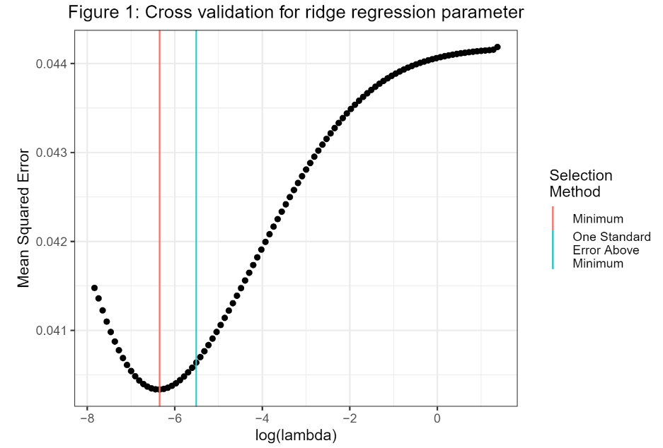
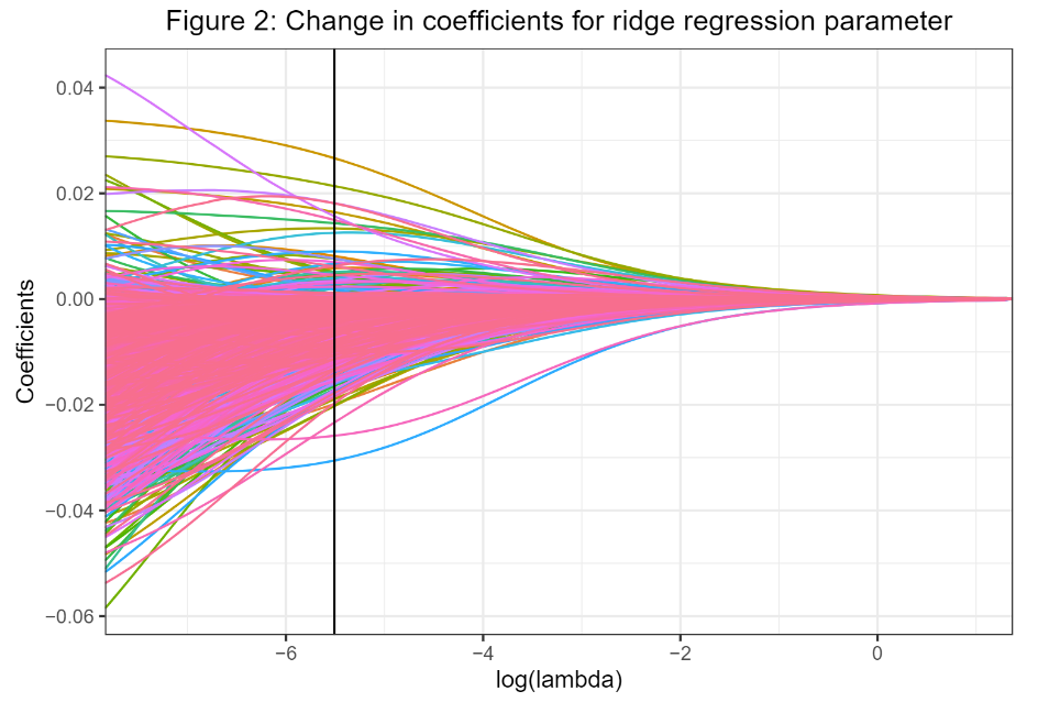
Using this value of $\lambda$ , we were then able to use the ridge regression solution to compute the model estimates $\boldsymbol{x}$ corresponding to each variable in $\boldsymbol{A}$ . The effect of $\log(\lambda)$ on the model coefficients can be seen in Figure 2, where a vertical line denotes our chosen ridge parameter. The reduction in variance and the shrinkage towards zero of the model coefficients as $\log(\lambda)$ increases can be seen in this graph.

Results

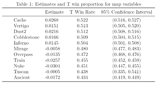
The ridge regression model’s coefficients for map are shown in Table 1 along with the average T side win percentage on that map.

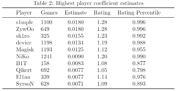
The coefficients for the remaining variables represent the estimated impact of each player in the model. The players with the ten highest coefficient estimates are shown in Table 2. We included their HLTV ratings and the corresponding percentile based on the rating as a way to compare the model results.

We explored the relationship between the coefficient estimates and the HLTV player ratings that were used as prior information in the model. Figure 3 shows a plot of a player’s average HLTV rating versus their coefficient estimate among players with at least 300 games played.

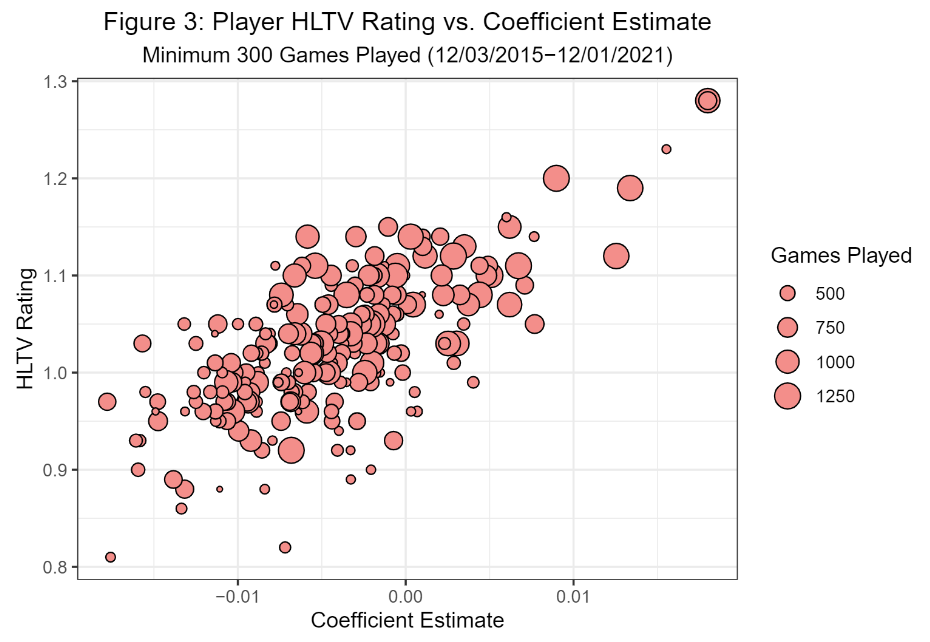
The correlation coefficient between rating and coefficient estimate was found to be 0.684 for these points, and the weighted correlation coefficient with games played as the weight for all points was found to be 0.658.

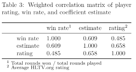
We also examined the relationship between the aforementioned HLTV rating and coefficient estimate with a player’s overall win rate in the time frame of interest. A weighted correlation matrix (weighted on games played) between these three variables is shown in Table 3.

Discussion

The map coefficient estimates in Table 1 are clearly related with the proportion of rounds won by the T side in the data set. If the T side has a win proportion of greater than 0.5 on any given map, the coefficient estimate is positive. Otherwise if the T side has a win proportion below 0.5, the corresponding estimate for that map is negative. The absolute value of the coefficient estimate depends on the difference between the proportion and 0.5, along with the proportion’s confidence interval. The 95% confidence interval was computed for the proportion of rounds won by the T side on each map (tWinPct) and the size of the interval varies based on how high the sample size is for each map. The map Tuscan has a massive 95% confidence interval for tWinPct from 0.335 to 0.541 because the map was only played in eight games (a total of 89 rounds), so it also has the coefficient estimate closest to zero.

The remaining model coefficient estimates represent the estimated impact of each player. As shown in Table 2, we’ve found that seven of the players with a top ten coefficient estimate also had an HLTV rating in at least the 95th percentile. The players with the five highest HLTV ratings (minimum 100 maps played) are all in the top six for coefficient estimates: s1mple, ZywOo, sh1ro, device, and NiKo. Oleksandr “s1mple” Kostyliev, Nicolai “device” Reedtz, and Nikola “NiKo” Kovač are all regarded as some of the greatest CS:GO players of all-time, while Mathieu “ZywOo” Herbaut and Dmitriy “sh1ro” Sokolov are young stars who are considered top five players in the world today. These claims seem to be supported by the players’ statistical dominance.

The weighted correlation matrix of player rating, win rate, and coefficient estimate (Table 3) suggests that the model estimates blend together both contribution to winning (0.609) and individual performance (0.658) in a way that neither metric can do on their own. By being able to combine both intertwined aspects of the game, teams can identify players that put up “empty stats” (racking up a high number of eliminations, but not contributing as much to their team’s winning chances) or players that quietly impact the game more than their basic statistics suggest.

Regularization has previously been used in a similar way for player evaluation in the National Basketball Association (Sill, 2010) and the same methodology appears to be applicable to an e-sports context. Future research should begin to explore the predictive capabilities of a regularization framework and continue to expand the use of advanced statistical methods in e-sports. Our regularization methodology can also be altered to better handle players with fluctuating skill levels throughout the time frame covered in the data set. For example, a player who peaked at a high skill level and then regressed later on would be treated as a single variable despite having varying impact throughout the data set. Also, the map dummy variables do not account for updates to each map that have taken place over the past years – these updates can affect the impact each map has on the terrorist team’s win rate. Despite the room for improvement, we believe that our research is a strong starting point for more advanced methods of player evaluation in e-sports.

References

Friedman, J. H., T. Hastie, and R. Tibshirani. “Regularization Paths for Generalized Linear Models via Coordinate Descent”. Journal of Statistical Software, vol. 33, no. 1, Feb. 2010, pp. 1-22, doi:10.18637/jss.v033.i01.
Milovanovic, P. (2017, June 14). Introducing rating 2.0. HLTV.org. Retrieved December 6, 2021, from https://www.hltv.org/news/20695/introducing-rating-20.
Sill, Joseph. “Improved NBA adjusted +/- using regularization and out-of-sample testing.” Proceedings of the 2010 MIT sloan sports analytics conference. 2010.