Icing the Kicker: A Python Analysis

It’s a scenario we’ve seen time and time again. With less than 10 seconds left in regulation, the team with possession lines up for what could be a game-winning field goal. The outcome of the game comes down to a single kick. The opposing coach can do nothing but stand on the sideline and pray that the kick is either blocked or the kicker simply misses. Well, they actually have one other option: calling a timeout. This tactic, known as ‘icing the kicker,’ is meant to mentally disrupt the opposing kicker and hopefully cause him to make a mistake. It’s a long shot, but it’s really all you can do at that point. The question: does it work?

I’ll conduct this experiment using nothing but Python. Everything done in this article will be reproducible using just the code presented here. If you just want an answer to the question and aren’t interested in the code, click here to jump to the conclusion.

First, I obviously need data to analyze. Here’s some simple code that can be used to create a Pandas DataFrame containing play-by-play logs for every regular season and postseason game prior to the current 2019 postseason. Credit to the nflscrapR team for compiling this data.

### preliminary imports
import matplotlib.pyplot as plt
from scipy import stats
import pandas as pd
import numpy as np

df_list = []

### get regular season logs
for yr in [2009,2010,2011,2012,2013,2014,2015,2016,2017,2018,2019]:
    url = 'https://raw.githubusercontent.com/ryurko/nflscrapR-data/master/play_by_play_data/regular_season/reg_pbp_' + str(yr) + '.csv'
    df = pd.read_csv(url,index_col=0,parse_dates=[0])
    df_list.append(df)

### get postseason logs
for yr in [2009,2010,2011,2012,2013,2014,2015,2016,2017,2018]:
    url = 'https://raw.githubusercontent.com/ryurko/nflscrapR-data/master/play_by_play_data/post_season/post_pbp_' + str(yr) + '.csv'
    df = pd.read_csv(url,index_col=0,parse_dates=[0])
    df_list.append(df)  
    
### combine
full_pbp = pd.concat(df_list).reset_index(drop=True)

Now we have a dataset full_pbp with data for every NFL play since 2009. Let’s see just how large the dataset is.

full_pbp.shape

(519520, 255)

Over half a million rows consisting of 255 columns. That’s a lot. It would be a good idea to create a second DataFrame with just the columns we’ll actually work with.

pbp = full_pbp[['home_team','posteam','score_differential','qtr','kick_distance','field_goal_result','timeout','timeout_team']]

I created a separate DataFrame instead of just editing the original one because if I made a mistake while editing it (like realizing I want more columns than the ones I selected), I would have to waste a lot of time reloading the original DataFrame.

The timeout column is a binary indicator (0 or 1) for whether there was a timeout called. However, there is a separate row for every timeout — it doesn’t tell us whether there was a timeout called before a given play.

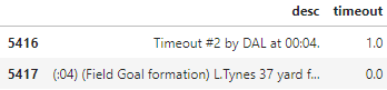
I want the 1 in the timeout column to be on the same row as the field goal play, so I’ll shift the entire timeout column down a single row. Same with the timeout_team column.

pbp['timeout'] = pbp.timeout.shift(1)
pbp['timeout_team'] = pbp.timeout_team.shift(1)

Now that we’ve identified plays in which timeouts were called prior to the snap, we can drop all of the rows in pbp that don’t represent field goal attempts. The field_goal_result column contains a value of NaN if there was not a field goal attempt on a given play, so we can just keep the rows that don’t contain NaN in field_goal_result.

pbp = pbp[~pbp.field_goal_result.isna()].reset_index(drop=True)

And now let’s check the size of our trimmed dataset:

pbp.shape

(11281, 8)

That’s much better than 519,520 rows and 255 columns.

Now that we have all of the data we need, we should make sure the data is in the correct form. Let’s take a look at what a snippet of pbp actually looks like.

pbp.head()

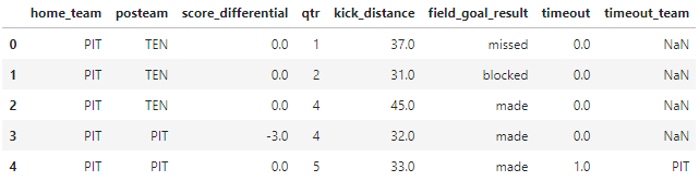
It’s nice that our data tells us specifically whether a kick is missed because it was blocked. However, this isn’t relevant to our analysis. All we care about is whether the field goal is good or no good. So, let’s convert this column into binary form.

pbp.field_goal_result.replace(['missed','blocked','made'], [0,0,1], inplace=True)

This code replaces each of the three possibilities for the field_goal_result column with numeric values. A 1 represents a successful field goal, while a value of 0 represents a missed field goal.

We also need a column which serves as a binary indicator for whether or not the kicker was iced on a given field goal. We’ll define an icing as a field goal in which a timeout was called prior to the snap by the opposing team.

ind = np.where((pbp.timeout == 1) & (pbp.timeout_team != pbp.posteam))[0]
pbp['iced'] = 0
for i in ind:
    pbp.iced[i] = 1

The first line of code outputs an array ind with the indices for every row in which the conditions are met for an iced kicker. Then, the column iced is initialized and filled with 0. The for loop is used to replace that 0 with a 1 at the previously identified indices.

Great. Now, we also need to create a column that tells us whether or not a given kick is a high-pressure field goal. After all, kickers are typically iced on these kicks. Maybe field goal percentages drop on clutch kicks, and kickers also just happen to be iced more often on clutch kicks. If we don’t identify clutch kicks, we won’t know if the trend is due to the kicker being iced or just because it’s a high-pressure kick, which are kicks in which kickers are more likely to be iced.

ind = np.where(((pbp.score_differential >= -3) & (pbp.score_differential <= 0)) & ((pbp.qtr / 4) >= 1))[0]
pbp['clutch'] = 0
for i in ind:
    pbp.clutch[i] = 1

The same exact technique that was used for the iced column was used to create this clutch column. I defined a high-pressure field goal as a field goal in the 4th quarter or overtime to either tie the game or go-ahead.

One more potential confounding variable to take care of: home-field advantage. We’ll just create a column that will serve as a binary indicator for whether the home team are the ones kicking.

def home(hometeam,posteam):
    if hometeam == posteam:
        return 1
    else:
        return 0
pbp['home'] = np.vectorize(home)(pbp.home_team, pbp.posteam)

I used a bit of a different technique this time because for some reason, the np.where method took ages to complete this task, while np.vectorize was instantaneous.

Now, let’s remove the columns we used to create the iced and clutch columns because they are no longer needed. I’ll also rename a couple of columns just so the names are shorter.

pbp = pbp[['kick_distance','field_goal_result','iced','clutch','home']]
pbp.columns = ['distance','made','iced','clutch','home']

While we’re at it, let’s take a peek at what a snippet of pbp looks like now.

pbp.head()

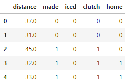
Excellent! All of our data is now numeric. Well, almost. there’s a NaN value for distance in eight of the 11,281 rows of pbp. I’ll just cut my losses and drop those rows.

pbp = pbp.dropna()

Now, it’s time to actually try and answer our initial question: does icing the kicker work?

Let’s start off by taking an elementary look at a conditional mean DataFrame grouped by the iced column.

pbp.groupby('iced').mean()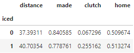

Since 2009, kickers hit 6.18% less of their field goal attempts when the opposing team called a timeout prior to the snap. So we’ve solved the question, right? Not quite. This data also tells us that the average ‘iced’ field goal is also over 3 yards longer and the 18.79% more likely to be a high-stakes kick. We can’t draw any conclusions without accounting for these variables.

I already proved in my previous article that kickers are less accurate at greater distances (shocking development, I know):

This very basic model can be used to calculate a probability of success for a field goal attempt based on distance. Here’s how we can create it from scratch:

means = pd.DataFrame(pbp.groupby('distance')['made'].mean()).reset_index(drop=False)
x = means.distance
y = means.made

trend = np.poly1d(np.polyfit(x,y,3))
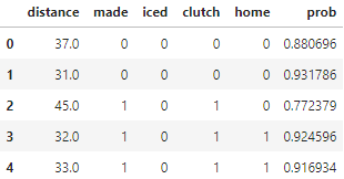
pbp['xfg_pct'] = trendpoly(pbp['distance'])

First, the means DataFrame is created, which consists of two columns: distance and made. The made simply has the average field goal percentage for every distance. These two variables can be used to fit a polynomial model to the data and use it to create a prob column for the probability of a given field goal to be successful. So, this is what pbp looks like now:

pbp.head()

Great. Now, I think we can analyze the effect of icing the kicker by accounting for the two lurking variables: the distance of a field goal and whether it’s a high-pressure situation. I’m not including home-field advantage because the previous conditional mean DataFrame showed that there is not a significant difference in home-field advantage when a kicker is or isn’t iced (unsurprisingly). I’ll just drop that column now, right before I create another conditional mean DataFrame after our adjustments.

pbp = pbp[['distance','made','iced','clutch','prob']]
pbp[pbp.clutch == 1].groupby('iced').mean()

In the second line, we’re once again creating a conditional mean DataFrame grouped by the iced column. However, this time we’re only looking at plays where the value in the clutch column is 1. Our polynomial model is accounting for distance, and now we can account for high-pressure situations by only looking at clutch field goals. Let’s take a look at the output.

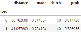
On field goals to tie the game or go-ahead in the 4th quarter or overtime, a kicker’s probability of success is 5.29% lower than expected based on distance if a timeout is called prior to the snap. Otherwise, the probability of a made field goal is just 0.29% lower than expected. It appears that kickers don’t really become less accurate if the stakes are high — they become less accurate if they’re iced.

Is this statistically significant? A t-test can answer that for us.

d1 = pbp[(pbp.clutch == 1) & (pbp.iced == 0)].made
d2 = pbp[(pbp.clutch == 1) & (pbp.iced == 1)].made
p_val = stats.ttest_ind(d1,d2)[1]
print('p-value: ' + str(p_val))

p-value: 0.017371021957504926

The p-value is less than 0.05, so we can reject the null hypothesis that icing the kicker does not have an impact on the success rate of field goals.

Keep calling those timeouts, NFL coaches. Just hope you time it correctly and you don’t end up giving the kicker a free practice swing.